#> # A tibble: 6 × 3
#>   department  year rd_budget_mil
#>   <chr>      <dbl>         <dbl>
#> 1 DOD         1976         35696
#> 2 NASA        1976         12513
#> 3 DOE         1976         10882
#> 4 HHS         1976          9226
#> 5 NIH         1976          8025
#> 6 NSF         1976          2372
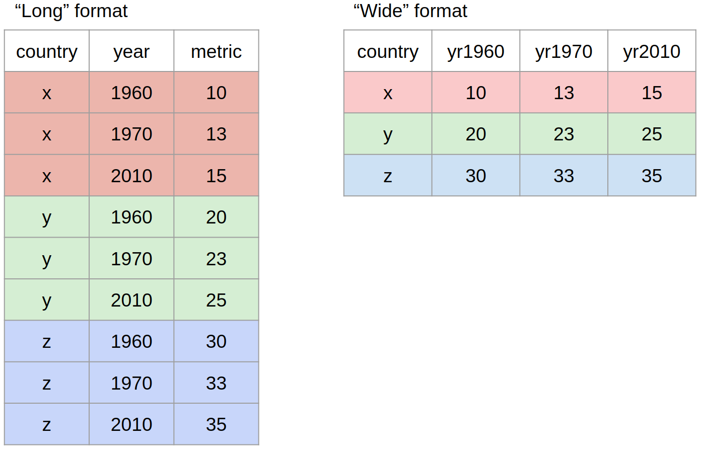
This is the same dataset, but in long format, where each observation has its own row. Here you will notice that the department names are now variables, and the R&D spending is a single column. The year is repeated for each department.
How do we know which format a dataset is in?
A helpful heuristic is to ask yourself:
Do the names describe the values?
If Yes: “Long” format
If No: “Wide” format
3.2 Tidy data = “Long” format
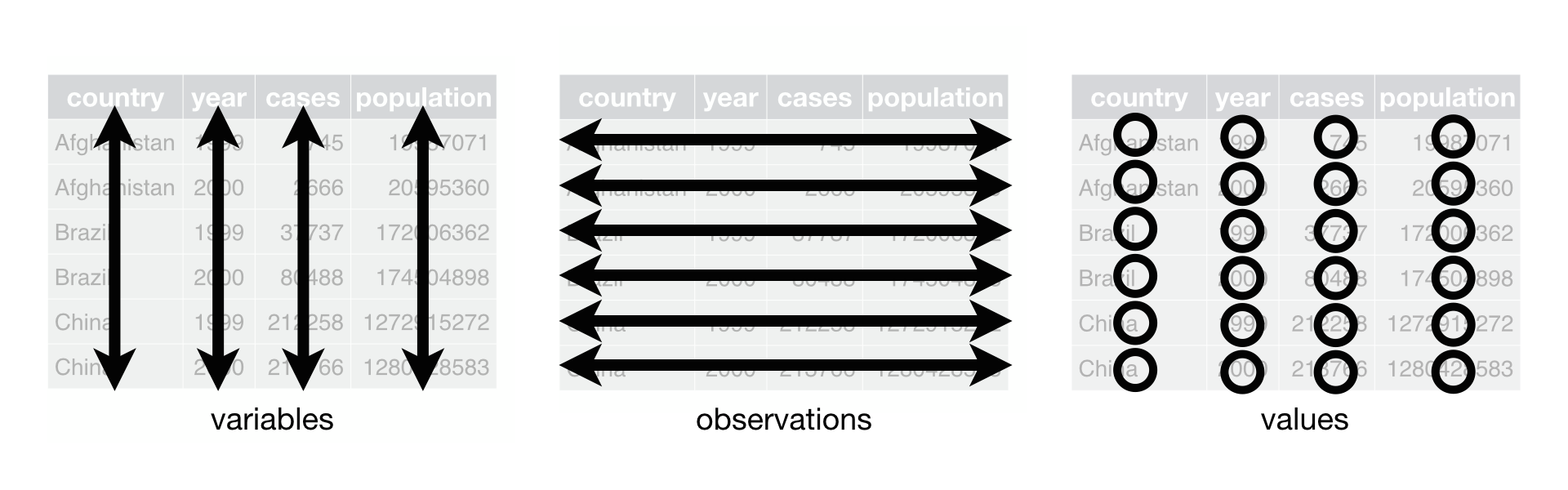
When we refer to “tidy data”, we are referring to data in long format that follows the “tidy” principles:
Each variable has its own column
Each observation has its own row
You can verify that the federal spending dataset is in long format:
head(fed_spend_long)
#> # A tibble: 6 × 3
#>   department  year rd_budget_mil
#>   <chr>      <dbl>         <dbl>
#> 1 DOD         1976         35696
#> 2 NASA        1976         12513
#> 3 DOE         1976         10882
#> 4 HHS         1976          9226
#> 5 NIH         1976          8025
#> 6 NSF         1976          2372
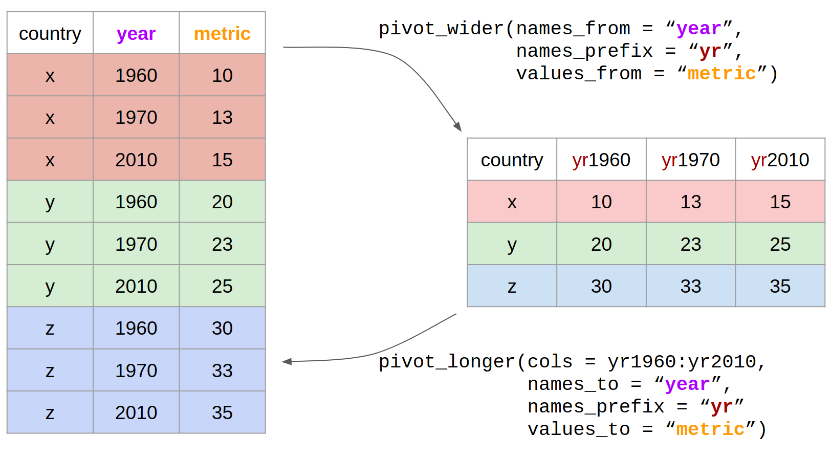
3.3 Reshaping data
We use the pivot_longer() and pivot_wider() functions to reshape data between long and wide formats.
#> # A tibble: 6 × 3
#>    year department rd_budget_mil
#>   <dbl> <chr>              <dbl>
#> 1  1976 DOD                35696
#> 2  1976 NASA               12513
#> 3  1976 DOE                10882
#> 4  1976 HHS                 9226
#> 5  1976 NIH                 8025
#> 6  1976 NSF                 2372
3.4 Tidy data wrangling
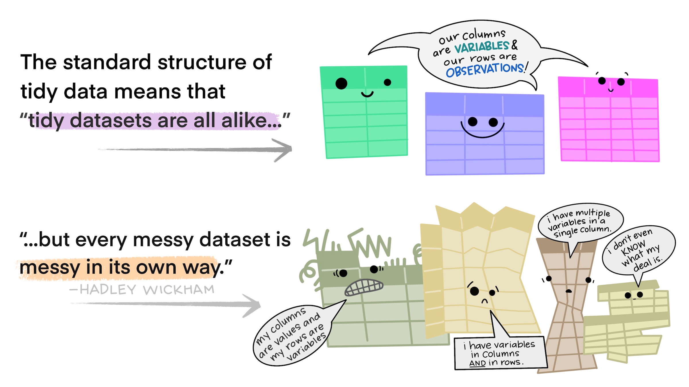
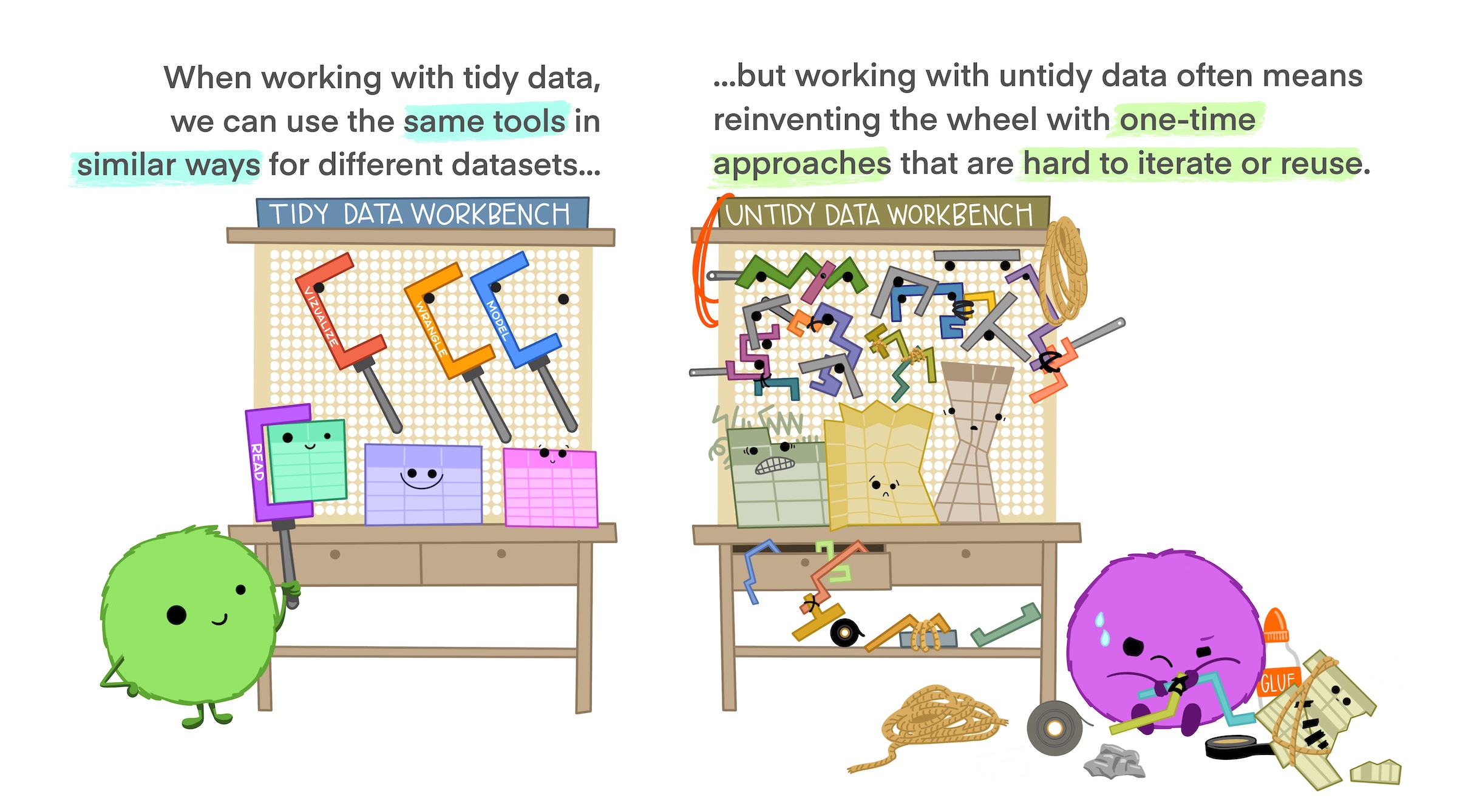
There’s a good reason why we like to keep our data in a long (tidy) format: it lets us use a consistent set of functions for manipulating, summarizing, and visualizing data.
Here’s a quick explanation with cute graphics, by Allison Horst:
3.4.1 Example 1: Total R&D spending in each year
This is a simple enough task, but with our data in wide format, we need to add each column manually like this:
fed_spend_wide %>%mutate(total = DHS + DOC + DOD + DOE + DOT + EPA + HHS + Interior + NASA + NIH + NSF + Other + USDA + VA) %>%select(year, total)
An alternative approach is to embrace the tidy data format. We’ll use pivot_longer() to convert the data into long format first, and then we’ll summarise the data:
#> Error in `geom_col()`:
#> ! Problem while computing aesthetics.
#> ℹ Error occurred in the 1st layer.
#> Caused by error:
#> ! object 'rd_budget_mil' not found
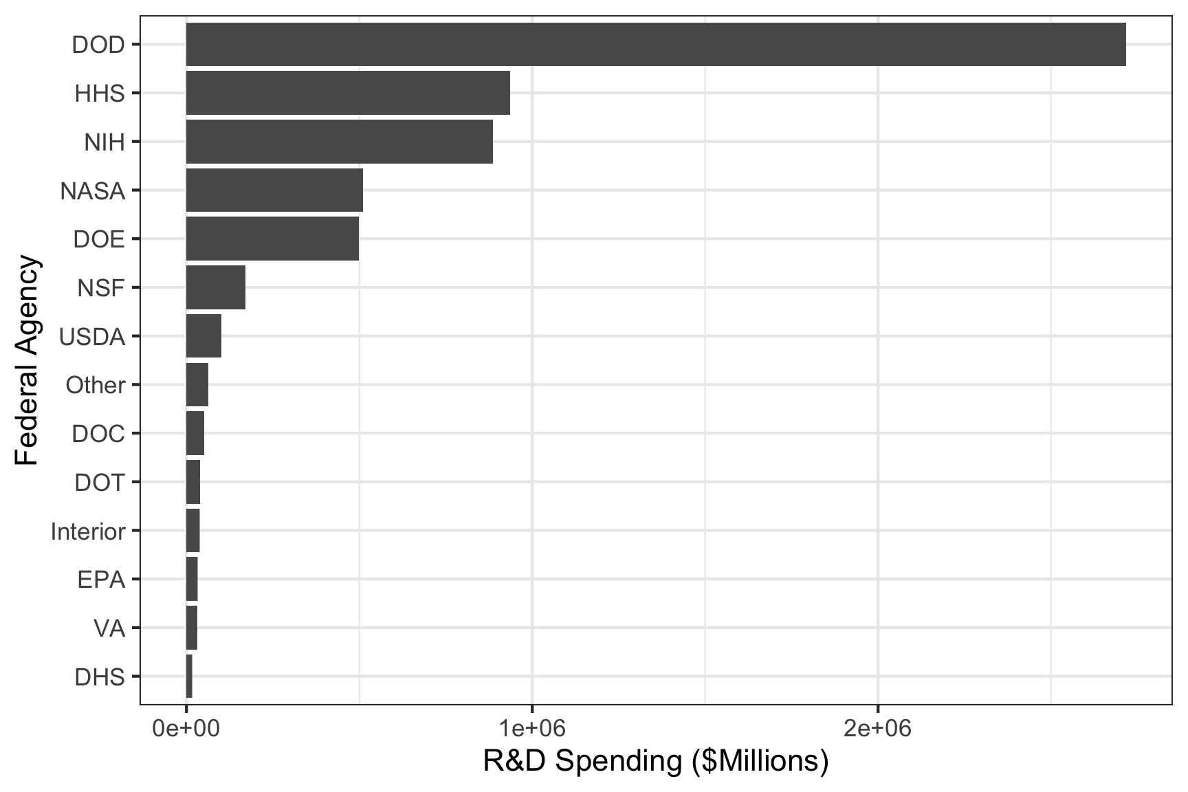
In wide format, we actually cannot plot the total by department, because there is no department variable!
Here we must first convert to long format, and then we can plot the data: